Statefulness#
In this tutorial we demonstrate how to train a stateful model in the KnowIt environment.
A stateful model is one that maintains an internal (or hidden) state across batches.
This is useful (and necessary) for building models that need to take into account long term dependencies in the data.
Specifically, dependencies that reach beyond the in_chunk of the time series model cannot be learned without
maintaining information from one batch to the next since batch features are always fixed length and of the shape:
- x[batch size, size of in_chunk, number of input components]
- y[batch size, size of out_chunk, number of output components]
By default KnowIt performs time series modeling in a stateless format,
where time is guaranteed to be contiguous within prediction points (across the second dimension in x and y), but not across batches.
To train a stateful model the user should provide the kwarg data_args['batch_sampling_mode'] = 'sliding-window'.
This tells KnowIt that batches should be constructed in a way so that time is also contiguous across batches.
How the model manages this statefulness is defined in the model architecture. See the default architecture LSTMv2 for
an example of an LSTM architecture with stateful capabilities.
The following sections provide further details in the form of a tutorial on simple stateful training.
1. Compile dataset #
First we need a simple dataset for which we know the underlying function.
We define a simple univariate running average y(t) = 0.5(x(t) + x(t-1)) where x ∈ U(0, 1).
This can be defined with the following method, given k = 1. In other words,
y at any given point in time is the average between x at the same point in time
and x at the preceding point in time.
# import numpy
import numpy as np
# set a random seed for reproducibility
np.random.seed(123)

# define data generating method
def generate_running_average_data(n, k):
    x = np.random.uniform(0, 1, n)
    y = []
    for t in range(n):
        y.append(0.5 * (x[t-k] + x[t]))
    y = np.array(y)
    return x, y
Next, we define a method to compile the data into a dataframe for
importing into KnowIt. Note that we simulate a time delta of
one millisecond between timesteps.
# import pandas
import pandas as pd
# import the datetime library
import datetime

# define data compiler method
def compile_dataframe(data_name, x, y, component_names):
    # convert the input and output components to two column vectors
    seq_data = np.array([x, y]).transpose()
    # define the time delta between time steps
    freq = datetime.timedelta(milliseconds=1)
    # define a range of datetime indices
    start = datetime.datetime.now()
    end = start + datetime.timedelta(milliseconds=len(x))
    t_range = pd.date_range(start, end, freq=freq)[:len(x)]
    # compile the dataframe
    new_frame = pd.DataFrame(seq_data, index=t_range, columns=component_names)
    # add the required meta data
    meta_data = {'name': data_name,
                 'components': component_names,
                 'time_delta': freq}
    new_frame.attrs = meta_data
    return new_frame
Using the two methods above, we can generate, compile, store, and visualize the dataset with the following code.
Note that our generated dataset consists of 10 000 timesteps and we called it k1_running_average.
# import matplotlib for visualization
import matplotlib.pyplot as plt

x, y = generate_running_average_data(n=10000, k=1)
new_frame = compile_dataframe(data_name='k1_running_average',
                              x=x,
                              y=y,
                              component_names=['x', 'y'])
new_frame.to_pickle(path='k1_running_average.pickle')

new_frame.plot()
plt.show()
plt.close()
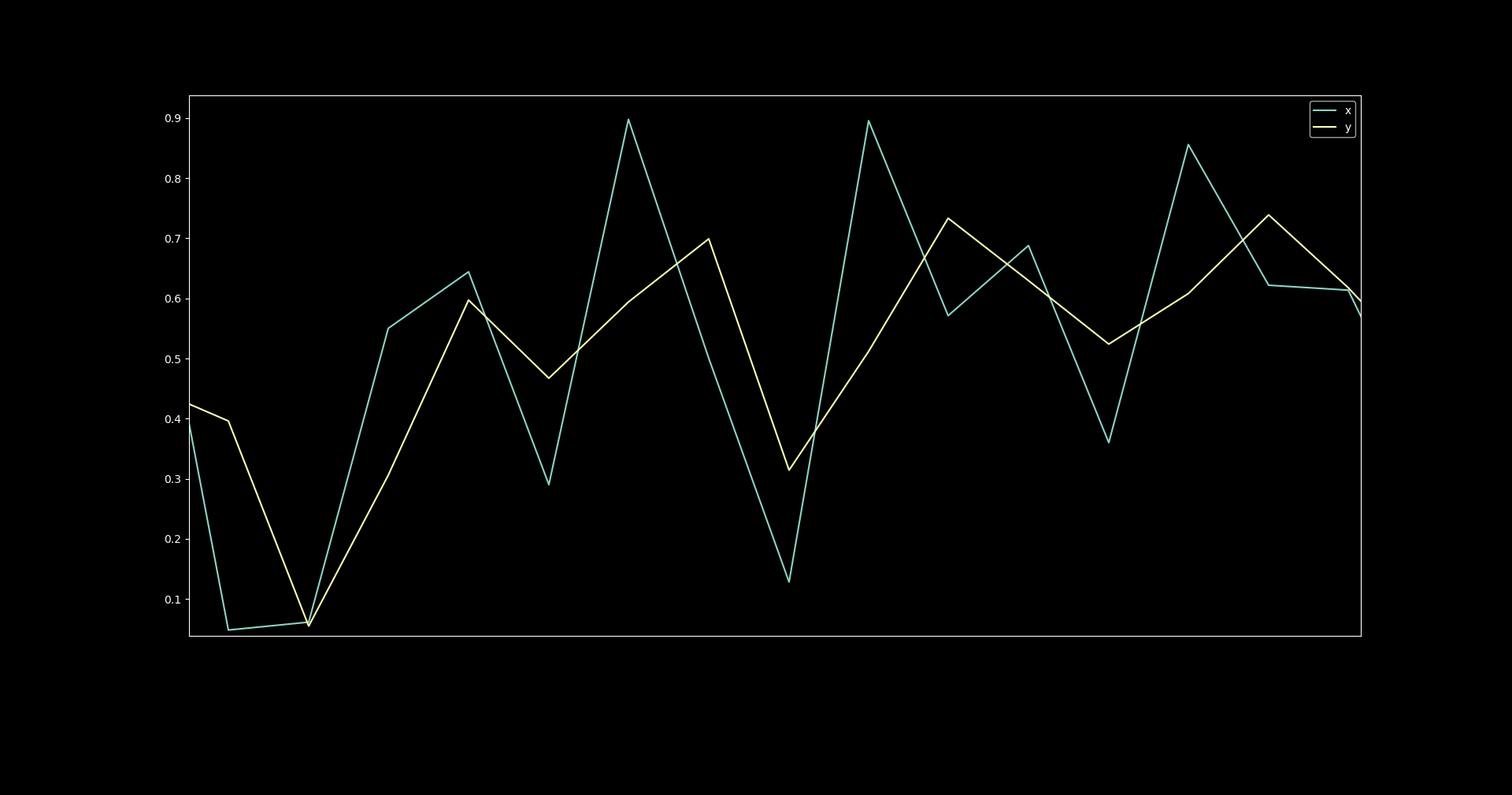
The resulting dataset shows no discernible pattern when
visualized as a whole.
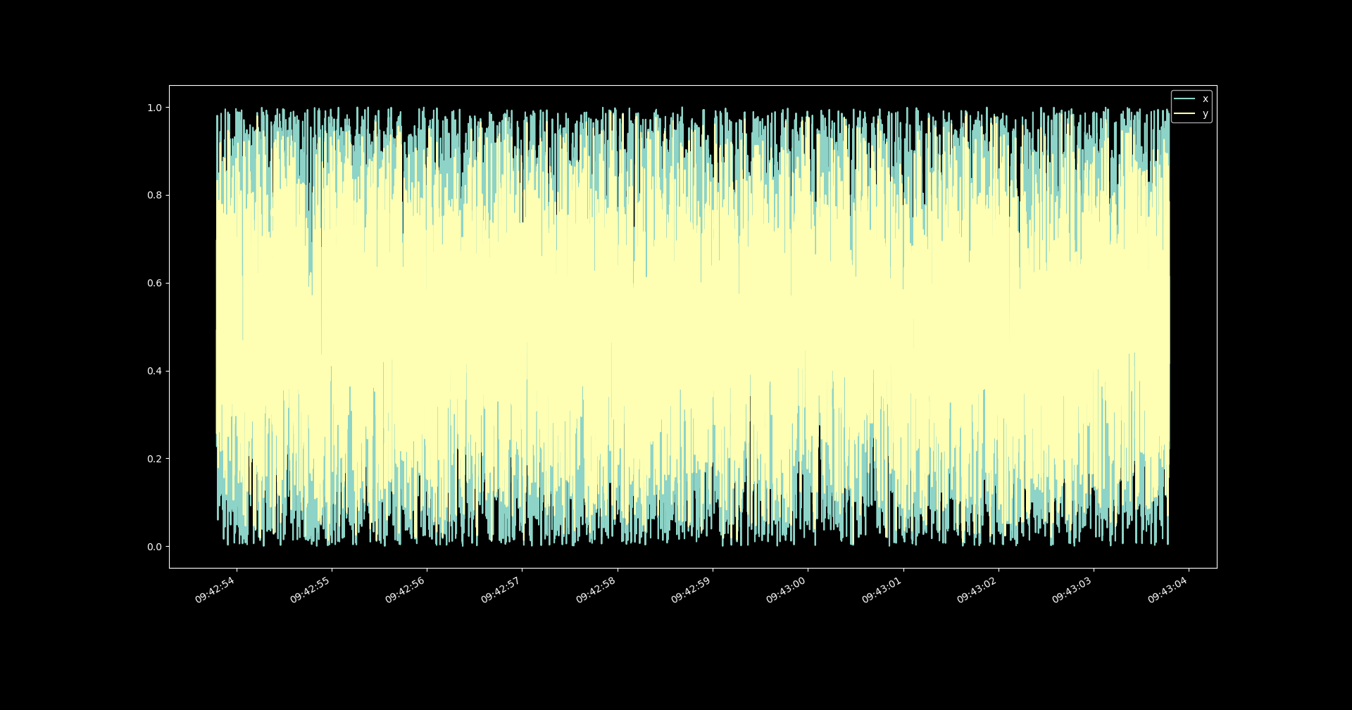
However, when we zoom in, we can see that each value for y
is the halfway point between the current x and the preceding one.
2. Set up baseline model building protocol #
Now that we have an imported dataset k1_running_average, we would like to train a time series model of
y(x). To do this we first need to define a couple of kwargs.
The basic kwargs for model training are data, arch, and trainer.
We define a nifty method get_basic_kwargs to produce these kwargs below.
In order to keep things simple we first construct our task as predicting y(t) given
x(t). We know that a model that can only consider x(t) to produce y(t) will be unable
to fit the true underlying function y(t) = 0.5(x(t) + x(t-1)). We also select the default
architecture MLP, which produces a stateless model by design.
See the Basics tutorial for an explanation of the other kwargs.
def get_basic_kwargs(data_name):
    # define the data related arguments
    data_args = {'name': data_name,
                 'task': 'regression',
                 'in_components': ['x'],
                 'out_components': ['y'],
                 'in_chunk': [0, 0],
                 'out_chunk': [0, 0],
                 'split_portions': [0.6, 0.2, 0.2],
                 'batch_size': 16,
                 'scaling_tag': 'full'}

    # define your architecture
    arch_args = {'task': 'regression',
                 'name': 'MLP'}

    # define your trainer
    trainer_args = {'loss_fn': 'mse_loss',
                    'optim': 'Adam',
                    'max_epochs': 50,
                    'learning_rate': 0.0001,
                    'task': 'regression'}

    return data_args, arch_args, trainer_args
We also construct an instance of KnowIt connected to a new experiment output
directory stateful_tut_exp and import the newly constructed dataset.
# import the KnowIt class
from knowit import KnowIt

# create an instance of KnowIt connected to an experiment output directory
KI = KnowIt(custom_exp_dir='stateful_tut_exp')
# switch on visualisation by default
KI.global_args(and_viz=True)
# import the raw dataset
KI.import_dataset({'data_import': {'raw_data': 'k1_running_average.pickle'}})
Finally, we define a method to train the model and produce predictions on the
validation set, for analysis.
def train_and_predict(model_name, data_args, arch_args, trainer_args):
    KI.train_model(model_name=model_name,
                   kwargs={'data': data_args,
                           'arch': arch_args,
                           'trainer': trainer_args})
    KI.generate_predictions(model_name=model_name,
                            kwargs={'predictor': {'prediction_set': 'valid'}})
Note that we have chosen to use an MLP-based model as our baseline.
We choose this architecture to first indicate the expected level of performance
when a completely stateless model is trained on the data.
This model has no hope of fitting the true underlying function since it is only
presented with the input component at the current point in time and has no mechanism of
remembering previous values. We can later compare the performance of a stateful model with
the performance of our baseline.
3. Train a baseline MLP #
All we need to do now is to call the get_basic_kwargs method, and send the resulting
kwargs to the train_and_predict method along with a model name.
Here we call our basline model simple_mlp.
data_args, arch_args, trainer_args = get_basic_kwargs('k1_running_average')
train_and_predict('simple_mlp', data_args, arch_args, trainer_args)
The resulting model obtained a best validation loss of 0.0204 at epoch 23 out of 50.
If we take a more qualitative look at its performance, through a zoomed in visualization of predictions on the
validation set, we see that the model was unable to fully capture the underlying function.
This is expected since we did not present the model with all the required inputs,
namely x(t) and x(t-1).

4. Train an MLP with extra history #
As a sanity check, we also train a model where we provide all the required inputs by adding
the time step preceding the current one to the model’s input chunk.
data_args, arch_args, trainer_args = get_basic_kwargs('k1_running_average')
data_args['in_chunk'] = [-1, 0]
train_and_predict('simple_oracle_mlp', data_args, arch_args, trainer_args)
The resulting model obtained a best validation loss of 0.0013 at epoch 14 out of 50.
Note that this model obtained a validation loss a magnitude lower than the baseline; it also
achieved this performance much earlier in training.
This is expected since the problem boils down to calculating the average between the two input features.
Through qualitative inspection, we also see that this model produces outputs much closer to the ground
truths on the validation set.

5. Stateful training #
Before training a stateful model, it would be prudent to explain some mechanisms used in Knowit.
5.1. Batch ordering #
When constructing batches in the default batch sampling mode, with data_args['batch_sampling_mode'] = 'independent',
each prediction point is packaged into batches
in an arbitrary order (prediction points are shuffled if data_args['shuffle_train'] = True).
If our dataset consists of 100 contiguous prediction points [1, 2, …, 99, 100],
and our batch size is 4, our first set of batches might look something like:
batch 1
batch 2
batch 3
…
35
28
29
…
67
96
86
…
7
88
1
…
3
43
55
…
Take note that, while the order of prediction points within and across batches are arbitrary, the
order of features corresponding to each prediction point will never be. The order of time steps
within a sequence corresponding to the input- and output-chunk of each prediction point will be
in the order that they appear in the base dataset (i.e. chronologically).
When constructing batches in the sliding-window mode, with data_args['batch_sampling_mode'] = 'sliding-window',
the CustomSampler ensures that a prediction point,
occupying a certain index in a batch follows contiguously after the prediction point that occupies
the same index in the preceding batch as far as possible.
To do this, a sliding window approach is taken. Each batch corresponds to a window of as many
prediction points as the batch size. The sliding window is then shifted by a slide_stride (default is 1)
prediction points to sample the next batch.
Continuing with the example above, our first set of batches might look something like:
batch 1
batch 2
batch 3
…
1
2
3
…
2
3
4
…
3
4
5
…
4
5
6
…
Note some key differences when comparing sliding-window and the default independent batch sampling mode.
For the latter, each prediction point will only appear once per epoch.
For the former, the number of times a prediction point
appears depends on the batch size, total number of prediction points, and the stride used.
Also note that the example above is only the general case. There are several edge cases
that are handled by the CustomSampler. These include:
If there are more than one slice in the dataset.
If there are more slices than batch size.
Whether data_args['shuffle_train'] is True or False.
The general algorithm for the sliding window approach is as follows. See CustomSampler for
exact details.
1. Get a list of all contiguous slices in the dataset split. These are lists of contiguous prediction points.
2. Shuffle the order of these slices if 'shuffle_train'=True.
3. If there are fewer slices than batch_size, add slices by duplicating and shifting existing ones until there are enough.
4. Shuffle the order of these expanded slices if 'shuffle_train'=True.
5. If 'shuffle_train'=True, drop a random number (between 0 and 10) of prediction points at the start of each slice.
6. If slide_stride > 1 subsample these expanded slices accordingly.
7. Iteratively sample batches from the slices in order to maintain as much contigousness across batch indices as possible.
8. Resulting batches that are smaller than batch size are dropped.
As a final note, for inference (i.e. validation, evaluation, prediction, and interpretation)
we use a third batch sampling mode called inference. This is always used for inference regardless of the
batch sampling mode selected for training. This sampling mode performs only steps 1, 6, and 7 above.
That means no shuffling or expansion is done, ensuring that all prediction points are sampled only once and are presented to
the model in order. It also means that if there are fewer slices in the dataset than batch size, the actual batch
size during inference will be smaller.
5.2. Handling states #
By selecting the sliding-window batch sampler as described in the previous section we ensure that the model
receives prediction points in the correct order for maintaining information across batches. However, as mentioned,
this is only done as far as possible. Some discontinuity is expected, especially with multiple slices and random
dropping if shuffling is used. This means that it would be unwise (and sometimes impossible) to maintain a single unbroken
hidden state throughout training. The hidden state should only be maintained when it makes sense (i.e. when the batches
follow each-other contiguously). Managing the hidden states falls on the architecture being trained.
Models in the KnowIt framework that have the ability to be stateful must have a force_reset() and update_states(...) method.
force_reset is called by the trainer module before each train, validation, or evaluation loop. It tells the architecture
to reset all its internal states so that no test set leakage occurs when moving into the new loop.
The update_states method receives a tensor of shape [batch size, 3]. It represents the IST indices of the prediction points
in the current batch. It can be used to monitor for breaks in contigiousness across batches.
See the internal method update_states in the default architecture LSTMv2 for an example of this.
Alternatively, if the architecture does not have the two methods above it is assumed to be stateless like
the default architecture MLP.
6. Train a stateful LSTM #
To demonstrate the capability of a stateful model we train a simple stateful LSTM on the same
dataset defined in Section 1. Note that we make some modifications to the model building protocol.
Namely, we select the sliding-window batch sampling mode, we select the LSTMv2
default architecture, and we train the model for longer. Additionally, we change some of the
default hyperparameters of LSTMv2 since this is a very simple dataset and would likely not require
most of the bells and whistles.
Importantly, we do not provide the model with x(t-1) by changing in_chunk. This means that
the model only observes x at the current point in time for each update.
data_args, arch_args, trainer_args = get_basic_kwargs('k1_running_average')
data_args['batch_sampling_mode'] = 'sliding-window'
arch_args['name'] = 'LSTMv2'
trainer_args['max_epochs'] = 100
arch_args['arch_hps'] = {'stateful': True,
                         'depth': 1,
                         'width': 32,
                         'residual': False,
                         'layernorm': False}
train_and_predict('simple_stateful_lstm_sliding-window', data_args, arch_args, trainer_args)
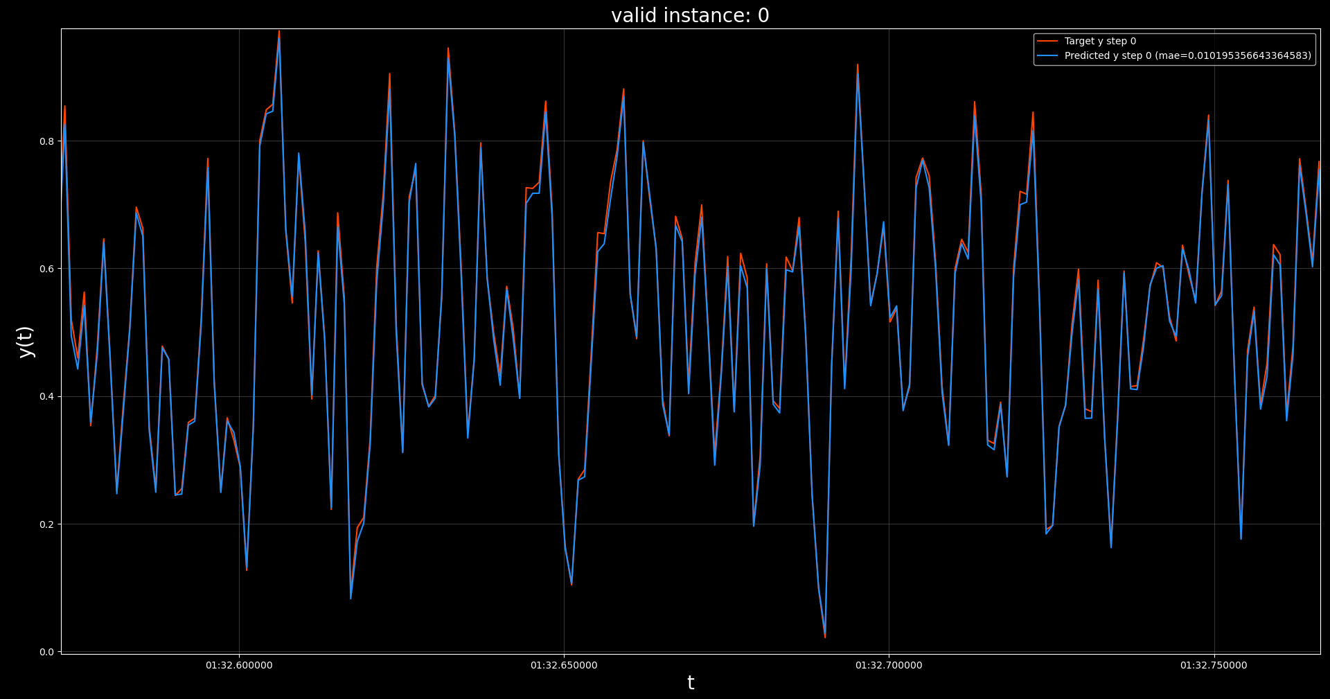
The resulting model obtained a best validation loss of 0.0010 at epoch 100 out of 100, although
it already reached a validation loss of 0.0052 before epoch 50.
This level of performance is similar to the MLP with extra history,
successfully fitting the true
underlying function, without having access to all the required
input features at each parameter update. This is only possible by maintaining and updating a hidden state across batches in contiguous order.
Also note the near perfect predictive performance on the validation set, as visualized
below.
7. Train a stateless LSTM #
As a second sanity check we repeat the previous experiment, but with a stateless LSTM.
This means that the hidden state will be reset each time a batch is passed through the model.
We do this by using an identical training setup, with the only difference being that we provide
the architecture argument stateful = False.
data_args, arch_args, trainer_args = get_basic_kwargs('k1_running_average')
data_args['batch_sampling_mode'] = 'sliding-window'
arch_args['name'] = 'LSTMv2'
trainer_args['max_epochs'] = 100
arch_args['arch_hps'] = {'stateful': False,
                         'depth': 1,
                         'width': 32,
                         'residual': False,
                         'layernorm': False}
train_and_predict('simple_stateful_lstm_sliding-window', data_args, arch_args, trainer_args)
The resulting model obtained a best validation loss of 0.0203 at epoch 4 out of 100.
This level of performance is similar to the baseline MLP.
This is expected since both models do not maintain a hidden state across batches, which we
have established is required to find the true underlying function.
8. “Long” term memory #
As a fun final experiment, we repeat the training of the stateful LSTM as defined in Section 6 for
varying levels of k in the data generating process. We also vary the first term in in_chunk;
let’s call it lb for “look back”.
This means that our data in each case is defined as y(t) = 0.5(x(t) + x(t-k)) where x ∈ U(0, 1),
and our model is observing [x(t-lb),..., x(t)] trying to predict y(t) at each point in time,
but maintaining a hidden state across contiguous batches.
We will also only train these models for 40 epochs to save time.
for k in range(1, 9):
    # give new dataset a name
    data_name = 'k' + str(k) + '_running_average'
    # generate new dataset
    x, y = generate_running_average_data(n=10000, k=k)
    # compile and store new dataset into dataframe
    new_frame = compile_dataframe(data_name=data_name,
                                  x=x,
                                  y=y,
                                  component_names=['x', 'y'])
    new_frame.to_pickle(path=data_name + '.pickle')
    # import new dataframe into KnowIt
    KI.import_dataset({'data_import': {'raw_data': data_name + '.pickle'}})
    for lb in range(0, k):
        # give new model a name
        model_name = 'simple_stateful_lstm_k_' + str(k) + '_lb_' + str(lb)
        # get the baseline kwargs
        data_args, arch_args, trainer_args = get_basic_kwargs(data_name)
        # update training protocol for stateful LSTM training
        data_args['batch_sampling_mode'] = 'sliding-window'
        arch_args['name'] = 'LSTMv2'
        trainer_args['max_epochs'] = 40
        data_args['in_chunk'] = [-lb, 0]
        arch_args['arch_hps'] = {'stateful': True,
                                 'depth': 1,
                                 'width': 32,
                                 'residual': False,
                                 'layernorm': False}
        # train the model
        train_and_predict(model_name, data_args, arch_args, trainer_args)
We list the resulting best validation losses of each of these models in the table below.
lb = 0
lb = 1
lb = 2
lb = 3
lb = 4
lb = 5
lb = 6
lb = 7
k=1
0.0057
xxxxxx
xxxxxx
xxxxxx
xxxxxx
xxxxxx
xxxxxx
xxxxxx
k=2
0.0071
0.0001
xxxxxx
xxxxxx
xxxxxx
xxxxxx
xxxxxx
xxxxxx
k=3
0.0176
0.0002
0.0002
xxxxxx
xxxxxx
xxxxxx
xxxxxx
xxxxxx
k=4
0.0188
0.0164
0.0004
0.0004
xxxxxx
xxxxxx
xxxxxx
xxxxxx
k=5
0.0206
0.0206
0.0166
0.0018
0.0003
xxxxxx
xxxxxx
xxxxxx
k=6
0.0204
0.0206
0.0207
0.0208
0.0204
0.0002
xxxxxx
xxxxxx
k=7
0.0206
0.0208
0.0210
0.0209
0.0207
0.0211
0.0154
xxxxxx
k=8
0.0205
0.0210
0.0212
0.0212
0.0211
0.0211
0.0213
0.0178
From the results we see that if our simple LSTM is only given
the current point in time x(t) as input,
it can find the true underlying function only if the required features are within
the first two preceding batches (see k=1 and k=2) in the lb=0 column.
Performance drops drastically as the required feature is moved further into the past.
We can make this observation for most of the lb values. If the important
feature x(t-k) is within the first two or three batches the model can find it and fit the function,
otherwise it defaults to a level of performance comparable to our stateless MLP in
Section 3.
This is except for lb=6 and lb=7. In these cases it seems our simple
LSTM cannot find the true function even if the required features are only one batch
into the past. This could either be due to a lack of capacity (there are more input features)
or simply a result of improper hyperparameters.
These results indicate that stateful training can learn patterns with longer dependencies
than defined by in_chunk, but it might still be worthwhile to use a larger in_chunk as well.
Disclaimer: A more rigorous experimental setup (HP tuning, mutliple seeds, etc.)
would be required if we want these conclusion to generalize. This is just a tutorial :)
9. Conclusion #
In this tutorial we used a very (very) simple dataset to demonstrate how stateful
training is handled in the KnowIt framework. In a real-world scenario you
usually do not know what input features are important and there is a lot more
hyperparameter tuning required to help your model find them.
The main takeaway is that if you suspect that the relevant information to make good
generalizable predictions are far apart in the time domain (farther than your in_chunk
can allow), it would be a good idea to consider stateful training.
First we need a simple dataset for which we know the underlying function.
We define a simple univariate running average y(t) = 0.5(x(t) + x(t-1)) where x ∈ U(0, 1).
This can be defined with the following method, given k = 1. In other words,
y at any given point in time is the average between x at the same point in time
and x at the preceding point in time.
# import numpy
import numpy as np
# set a random seed for reproducibility
np.random.seed(123)
# define data generating method
def generate_running_average_data(n, k):
x = np.random.uniform(0, 1, n)
y = []
for t in range(n):
y.append(0.5 * (x[t-k] + x[t]))
y = np.array(y)
return x, y
Next, we define a method to compile the data into a dataframe for
importing into KnowIt. Note that we simulate a time delta of
one millisecond between timesteps.
# import pandas
import pandas as pd
# import the datetime library
import datetime
# define data compiler method
def compile_dataframe(data_name, x, y, component_names):
# convert the input and output components to two column vectors
seq_data = np.array([x, y]).transpose()
# define the time delta between time steps
freq = datetime.timedelta(milliseconds=1)
# define a range of datetime indices
start = datetime.datetime.now()
end = start + datetime.timedelta(milliseconds=len(x))
t_range = pd.date_range(start, end, freq=freq)[:len(x)]
# compile the dataframe
new_frame = pd.DataFrame(seq_data, index=t_range, columns=component_names)
# add the required meta data
meta_data = {'name': data_name,
'components': component_names,
'time_delta': freq}
new_frame.attrs = meta_data
return new_frame
Using the two methods above, we can generate, compile, store, and visualize the dataset with the following code.
Note that our generated dataset consists of 10 000 timesteps and we called it k1_running_average.
# import matplotlib for visualization
import matplotlib.pyplot as plt
x, y = generate_running_average_data(n=10000, k=1)
new_frame = compile_dataframe(data_name='k1_running_average',
x=x,
y=y,
component_names=['x', 'y'])
new_frame.to_pickle(path='k1_running_average.pickle')
new_frame.plot()
plt.show()
plt.close()
The resulting dataset shows no discernible pattern when visualized as a whole.
However, when we zoom in, we can see that each value for y
is the halfway point between the current x and the preceding one.
2. Set up baseline model building protocol #
Now that we have an imported dataset k1_running_average, we would like to train a time series model of
y(x). To do this we first need to define a couple of kwargs.
The basic kwargs for model training are data, arch, and trainer.
We define a nifty method get_basic_kwargs to produce these kwargs below.
In order to keep things simple we first construct our task as predicting y(t) given
x(t). We know that a model that can only consider x(t) to produce y(t) will be unable
to fit the true underlying function y(t) = 0.5(x(t) + x(t-1)). We also select the default
architecture MLP, which produces a stateless model by design.
See the Basics tutorial for an explanation of the other kwargs.
def get_basic_kwargs(data_name):
# define the data related arguments
data_args = {'name': data_name,
'task': 'regression',
'in_components': ['x'],
'out_components': ['y'],
'in_chunk': [0, 0],
'out_chunk': [0, 0],
'split_portions': [0.6, 0.2, 0.2],
'batch_size': 16,
'scaling_tag': 'full'}
# define your architecture
arch_args = {'task': 'regression',
'name': 'MLP'}
# define your trainer
trainer_args = {'loss_fn': 'mse_loss',
'optim': 'Adam',
'max_epochs': 50,
'learning_rate': 0.0001,
'task': 'regression'}
return data_args, arch_args, trainer_args
We also construct an instance of KnowIt connected to a new experiment output
directory stateful_tut_exp and import the newly constructed dataset.
# import the KnowIt class
from knowit import KnowIt
# create an instance of KnowIt connected to an experiment output directory
KI = KnowIt(custom_exp_dir='stateful_tut_exp')
# switch on visualisation by default
KI.global_args(and_viz=True)
# import the raw dataset
KI.import_dataset({'data_import': {'raw_data': 'k1_running_average.pickle'}})
Finally, we define a method to train the model and produce predictions on the
validation set, for analysis.
def train_and_predict(model_name, data_args, arch_args, trainer_args):
KI.train_model(model_name=model_name,
kwargs={'data': data_args,
'arch': arch_args,
'trainer': trainer_args})
KI.generate_predictions(model_name=model_name,
kwargs={'predictor': {'prediction_set': 'valid'}})
Note that we have chosen to use an MLP-based model as our baseline.
We choose this architecture to first indicate the expected level of performance
when a completely stateless model is trained on the data.
This model has no hope of fitting the true underlying function since it is only
presented with the input component at the current point in time and has no mechanism of
remembering previous values. We can later compare the performance of a stateful model with
the performance of our baseline.
3. Train a baseline MLP #
All we need to do now is to call the get_basic_kwargs method, and send the resulting
kwargs to the train_and_predict method along with a model name.
Here we call our basline model simple_mlp.
data_args, arch_args, trainer_args = get_basic_kwargs('k1_running_average')
train_and_predict('simple_mlp', data_args, arch_args, trainer_args)
The resulting model obtained a best validation loss of 0.0204 at epoch 23 out of 50.
If we take a more qualitative look at its performance, through a zoomed in visualization of predictions on the
validation set, we see that the model was unable to fully capture the underlying function.
This is expected since we did not present the model with all the required inputs,
namely x(t) and x(t-1).
4. Train an MLP with extra history #
As a sanity check, we also train a model where we provide all the required inputs by adding
the time step preceding the current one to the model’s input chunk.
data_args, arch_args, trainer_args = get_basic_kwargs('k1_running_average')
data_args['in_chunk'] = [-1, 0]
train_and_predict('simple_oracle_mlp', data_args, arch_args, trainer_args)
The resulting model obtained a best validation loss of 0.0013 at epoch 14 out of 50.
Note that this model obtained a validation loss a magnitude lower than the baseline; it also
achieved this performance much earlier in training.
This is expected since the problem boils down to calculating the average between the two input features.
Through qualitative inspection, we also see that this model produces outputs much closer to the ground
truths on the validation set.
5. Stateful training #
Before training a stateful model, it would be prudent to explain some mechanisms used in Knowit.
5.1. Batch ordering #
When constructing batches in the default batch sampling mode, with data_args['batch_sampling_mode'] = 'independent',
each prediction point is packaged into batches
in an arbitrary order (prediction points are shuffled if data_args['shuffle_train'] = True).
If our dataset consists of 100 contiguous prediction points [1, 2, …, 99, 100],
and our batch size is 4, our first set of batches might look something like:
batch 1
batch 2
batch 3
…
35
28
29
…
67
96
86
…
7
88
1
…
3
43
55
…
Take note that, while the order of prediction points within and across batches are arbitrary, the
order of features corresponding to each prediction point will never be. The order of time steps
within a sequence corresponding to the input- and output-chunk of each prediction point will be
in the order that they appear in the base dataset (i.e. chronologically).
When constructing batches in the sliding-window mode, with data_args['batch_sampling_mode'] = 'sliding-window',
the CustomSampler ensures that a prediction point,
occupying a certain index in a batch follows contiguously after the prediction point that occupies
the same index in the preceding batch as far as possible.
To do this, a sliding window approach is taken. Each batch corresponds to a window of as many
prediction points as the batch size. The sliding window is then shifted by a slide_stride (default is 1)
prediction points to sample the next batch.
Continuing with the example above, our first set of batches might look something like:
batch 1
batch 2
batch 3
…
1
2
3
…
2
3
4
…
3
4
5
…
4
5
6
…
Note some key differences when comparing sliding-window and the default independent batch sampling mode.
For the latter, each prediction point will only appear once per epoch.
For the former, the number of times a prediction point
appears depends on the batch size, total number of prediction points, and the stride used.
Also note that the example above is only the general case. There are several edge cases
that are handled by the CustomSampler. These include:
If there are more than one slice in the dataset.
If there are more slices than batch size.
Whether data_args['shuffle_train'] is True or False.
The general algorithm for the sliding window approach is as follows. See CustomSampler for
exact details.
1. Get a list of all contiguous slices in the dataset split. These are lists of contiguous prediction points.
2. Shuffle the order of these slices if 'shuffle_train'=True.
3. If there are fewer slices than batch_size, add slices by duplicating and shifting existing ones until there are enough.
4. Shuffle the order of these expanded slices if 'shuffle_train'=True.
5. If 'shuffle_train'=True, drop a random number (between 0 and 10) of prediction points at the start of each slice.
6. If slide_stride > 1 subsample these expanded slices accordingly.
7. Iteratively sample batches from the slices in order to maintain as much contigousness across batch indices as possible.
8. Resulting batches that are smaller than batch size are dropped.
As a final note, for inference (i.e. validation, evaluation, prediction, and interpretation)
we use a third batch sampling mode called inference. This is always used for inference regardless of the
batch sampling mode selected for training. This sampling mode performs only steps 1, 6, and 7 above.
That means no shuffling or expansion is done, ensuring that all prediction points are sampled only once and are presented to
the model in order. It also means that if there are fewer slices in the dataset than batch size, the actual batch
size during inference will be smaller.
5.2. Handling states #
By selecting the sliding-window batch sampler as described in the previous section we ensure that the model
receives prediction points in the correct order for maintaining information across batches. However, as mentioned,
this is only done as far as possible. Some discontinuity is expected, especially with multiple slices and random
dropping if shuffling is used. This means that it would be unwise (and sometimes impossible) to maintain a single unbroken
hidden state throughout training. The hidden state should only be maintained when it makes sense (i.e. when the batches
follow each-other contiguously). Managing the hidden states falls on the architecture being trained.
Models in the KnowIt framework that have the ability to be stateful must have a force_reset() and update_states(...) method.
force_reset is called by the trainer module before each train, validation, or evaluation loop. It tells the architecture
to reset all its internal states so that no test set leakage occurs when moving into the new loop.
The update_states method receives a tensor of shape [batch size, 3]. It represents the IST indices of the prediction points
in the current batch. It can be used to monitor for breaks in contigiousness across batches.
See the internal method update_states in the default architecture LSTMv2 for an example of this.
Alternatively, if the architecture does not have the two methods above it is assumed to be stateless like
the default architecture MLP.
6. Train a stateful LSTM #
To demonstrate the capability of a stateful model we train a simple stateful LSTM on the same
dataset defined in Section 1. Note that we make some modifications to the model building protocol.
Namely, we select the sliding-window batch sampling mode, we select the LSTMv2
default architecture, and we train the model for longer. Additionally, we change some of the
default hyperparameters of LSTMv2 since this is a very simple dataset and would likely not require
most of the bells and whistles.
Importantly, we do not provide the model with x(t-1) by changing in_chunk. This means that
the model only observes x at the current point in time for each update.
data_args, arch_args, trainer_args = get_basic_kwargs('k1_running_average')
data_args['batch_sampling_mode'] = 'sliding-window'
arch_args['name'] = 'LSTMv2'
trainer_args['max_epochs'] = 100
arch_args['arch_hps'] = {'stateful': True,
'depth': 1,
'width': 32,
'residual': False,
'layernorm': False}
train_and_predict('simple_stateful_lstm_sliding-window', data_args, arch_args, trainer_args)
The resulting model obtained a best validation loss of 0.0010 at epoch 100 out of 100, although
it already reached a validation loss of 0.0052 before epoch 50.
This level of performance is similar to the MLP with extra history,
successfully fitting the true
underlying function, without having access to all the required
input features at each parameter update. This is only possible by maintaining and updating a hidden state across batches in contiguous order.
Also note the near perfect predictive performance on the validation set, as visualized
below.
7. Train a stateless LSTM #
As a second sanity check we repeat the previous experiment, but with a stateless LSTM.
This means that the hidden state will be reset each time a batch is passed through the model.
We do this by using an identical training setup, with the only difference being that we provide
the architecture argument stateful = False.
data_args, arch_args, trainer_args = get_basic_kwargs('k1_running_average')
data_args['batch_sampling_mode'] = 'sliding-window'
arch_args['name'] = 'LSTMv2'
trainer_args['max_epochs'] = 100
arch_args['arch_hps'] = {'stateful': False,
'depth': 1,
'width': 32,
'residual': False,
'layernorm': False}
train_and_predict('simple_stateful_lstm_sliding-window', data_args, arch_args, trainer_args)
The resulting model obtained a best validation loss of 0.0203 at epoch 4 out of 100.
This level of performance is similar to the baseline MLP.
This is expected since both models do not maintain a hidden state across batches, which we
have established is required to find the true underlying function.
8. “Long” term memory #
As a fun final experiment, we repeat the training of the stateful LSTM as defined in Section 6 for
varying levels of k in the data generating process. We also vary the first term in in_chunk;
let’s call it lb for “look back”.
This means that our data in each case is defined as y(t) = 0.5(x(t) + x(t-k)) where x ∈ U(0, 1),
and our model is observing [x(t-lb),..., x(t)] trying to predict y(t) at each point in time,
but maintaining a hidden state across contiguous batches.
We will also only train these models for 40 epochs to save time.
for k in range(1, 9):
# give new dataset a name
data_name = 'k' + str(k) + '_running_average'
# generate new dataset
x, y = generate_running_average_data(n=10000, k=k)
# compile and store new dataset into dataframe
new_frame = compile_dataframe(data_name=data_name,
x=x,
y=y,
component_names=['x', 'y'])
new_frame.to_pickle(path=data_name + '.pickle')
# import new dataframe into KnowIt
KI.import_dataset({'data_import': {'raw_data': data_name + '.pickle'}})
for lb in range(0, k):
# give new model a name
model_name = 'simple_stateful_lstm_k_' + str(k) + '_lb_' + str(lb)
# get the baseline kwargs
data_args, arch_args, trainer_args = get_basic_kwargs(data_name)
# update training protocol for stateful LSTM training
data_args['batch_sampling_mode'] = 'sliding-window'
arch_args['name'] = 'LSTMv2'
trainer_args['max_epochs'] = 40
data_args['in_chunk'] = [-lb, 0]
arch_args['arch_hps'] = {'stateful': True,
'depth': 1,
'width': 32,
'residual': False,
'layernorm': False}
# train the model
train_and_predict(model_name, data_args, arch_args, trainer_args)
We list the resulting best validation losses of each of these models in the table below.
lb = 0
lb = 1
lb = 2
lb = 3
lb = 4
lb = 5
lb = 6
lb = 7
k=1
0.0057
xxxxxx
xxxxxx
xxxxxx
xxxxxx
xxxxxx
xxxxxx
xxxxxx
k=2
0.0071
0.0001
xxxxxx
xxxxxx
xxxxxx
xxxxxx
xxxxxx
xxxxxx
k=3
0.0176
0.0002
0.0002
xxxxxx
xxxxxx
xxxxxx
xxxxxx
xxxxxx
k=4
0.0188
0.0164
0.0004
0.0004
xxxxxx
xxxxxx
xxxxxx
xxxxxx
k=5
0.0206
0.0206
0.0166
0.0018
0.0003
xxxxxx
xxxxxx
xxxxxx
k=6
0.0204
0.0206
0.0207
0.0208
0.0204
0.0002
xxxxxx
xxxxxx
k=7
0.0206
0.0208
0.0210
0.0209
0.0207
0.0211
0.0154
xxxxxx
k=8
0.0205
0.0210
0.0212
0.0212
0.0211
0.0211
0.0213
0.0178
From the results we see that if our simple LSTM is only given
the current point in time x(t) as input,
it can find the true underlying function only if the required features are within
the first two preceding batches (see k=1 and k=2) in the lb=0 column.
Performance drops drastically as the required feature is moved further into the past.
We can make this observation for most of the lb values. If the important
feature x(t-k) is within the first two or three batches the model can find it and fit the function,
otherwise it defaults to a level of performance comparable to our stateless MLP in
Section 3.
This is except for lb=6 and lb=7. In these cases it seems our simple
LSTM cannot find the true function even if the required features are only one batch
into the past. This could either be due to a lack of capacity (there are more input features)
or simply a result of improper hyperparameters.
These results indicate that stateful training can learn patterns with longer dependencies
than defined by in_chunk, but it might still be worthwhile to use a larger in_chunk as well.
Disclaimer: A more rigorous experimental setup (HP tuning, mutliple seeds, etc.)
would be required if we want these conclusion to generalize. This is just a tutorial :)
9. Conclusion #
In this tutorial we used a very (very) simple dataset to demonstrate how stateful
training is handled in the KnowIt framework. In a real-world scenario you
usually do not know what input features are important and there is a lot more
hyperparameter tuning required to help your model find them.
The main takeaway is that if you suspect that the relevant information to make good
generalizable predictions are far apart in the time domain (farther than your in_chunk
can allow), it would be a good idea to consider stateful training.
Now that we have an imported dataset k1_running_average, we would like to train a time series model of
y(x). To do this we first need to define a couple of kwargs.
The basic kwargs for model training are data, arch, and trainer.
We define a nifty method get_basic_kwargs to produce these kwargs below.
In order to keep things simple we first construct our task as predicting y(t) given
x(t). We know that a model that can only consider x(t) to produce y(t) will be unable
to fit the true underlying function y(t) = 0.5(x(t) + x(t-1)). We also select the default
architecture MLP, which produces a stateless model by design.
See the Basics tutorial for an explanation of the other kwargs.
def get_basic_kwargs(data_name):
# define the data related arguments
data_args = {'name': data_name,
'task': 'regression',
'in_components': ['x'],
'out_components': ['y'],
'in_chunk': [0, 0],
'out_chunk': [0, 0],
'split_portions': [0.6, 0.2, 0.2],
'batch_size': 16,
'scaling_tag': 'full'}
# define your architecture
arch_args = {'task': 'regression',
'name': 'MLP'}
# define your trainer
trainer_args = {'loss_fn': 'mse_loss',
'optim': 'Adam',
'max_epochs': 50,
'learning_rate': 0.0001,
'task': 'regression'}
return data_args, arch_args, trainer_args
We also construct an instance of KnowIt connected to a new experiment output
directory stateful_tut_exp and import the newly constructed dataset.
# import the KnowIt class
from knowit import KnowIt
# create an instance of KnowIt connected to an experiment output directory
KI = KnowIt(custom_exp_dir='stateful_tut_exp')
# switch on visualisation by default
KI.global_args(and_viz=True)
# import the raw dataset
KI.import_dataset({'data_import': {'raw_data': 'k1_running_average.pickle'}})
Finally, we define a method to train the model and produce predictions on the validation set, for analysis.
def train_and_predict(model_name, data_args, arch_args, trainer_args):
KI.train_model(model_name=model_name,
kwargs={'data': data_args,
'arch': arch_args,
'trainer': trainer_args})
KI.generate_predictions(model_name=model_name,
kwargs={'predictor': {'prediction_set': 'valid'}})
Note that we have chosen to use an MLP-based model as our baseline. We choose this architecture to first indicate the expected level of performance when a completely stateless model is trained on the data. This model has no hope of fitting the true underlying function since it is only presented with the input component at the current point in time and has no mechanism of remembering previous values. We can later compare the performance of a stateful model with the performance of our baseline.
3. Train a baseline MLP #
All we need to do now is to call the get_basic_kwargs method, and send the resulting
kwargs to the train_and_predict method along with a model name.
Here we call our basline model simple_mlp.
data_args, arch_args, trainer_args = get_basic_kwargs('k1_running_average')
train_and_predict('simple_mlp', data_args, arch_args, trainer_args)
The resulting model obtained a best validation loss of 0.0204 at epoch 23 out of 50.
If we take a more qualitative look at its performance, through a zoomed in visualization of predictions on the
validation set, we see that the model was unable to fully capture the underlying function.
This is expected since we did not present the model with all the required inputs,
namely x(t) and x(t-1).
4. Train an MLP with extra history #
As a sanity check, we also train a model where we provide all the required inputs by adding
the time step preceding the current one to the model’s input chunk.
data_args, arch_args, trainer_args = get_basic_kwargs('k1_running_average')
data_args['in_chunk'] = [-1, 0]
train_and_predict('simple_oracle_mlp', data_args, arch_args, trainer_args)
The resulting model obtained a best validation loss of 0.0013 at epoch 14 out of 50.
Note that this model obtained a validation loss a magnitude lower than the baseline; it also
achieved this performance much earlier in training.
This is expected since the problem boils down to calculating the average between the two input features.
Through qualitative inspection, we also see that this model produces outputs much closer to the ground
truths on the validation set.
5. Stateful training #
Before training a stateful model, it would be prudent to explain some mechanisms used in Knowit.
5.1. Batch ordering #
When constructing batches in the default batch sampling mode, with data_args['batch_sampling_mode'] = 'independent',
each prediction point is packaged into batches
in an arbitrary order (prediction points are shuffled if data_args['shuffle_train'] = True).
If our dataset consists of 100 contiguous prediction points [1, 2, …, 99, 100],
and our batch size is 4, our first set of batches might look something like:
batch 1
batch 2
batch 3
…
35
28
29
…
67
96
86
…
7
88
1
…
3
43
55
…
Take note that, while the order of prediction points within and across batches are arbitrary, the
order of features corresponding to each prediction point will never be. The order of time steps
within a sequence corresponding to the input- and output-chunk of each prediction point will be
in the order that they appear in the base dataset (i.e. chronologically).
When constructing batches in the sliding-window mode, with data_args['batch_sampling_mode'] = 'sliding-window',
the CustomSampler ensures that a prediction point,
occupying a certain index in a batch follows contiguously after the prediction point that occupies
the same index in the preceding batch as far as possible.
To do this, a sliding window approach is taken. Each batch corresponds to a window of as many
prediction points as the batch size. The sliding window is then shifted by a slide_stride (default is 1)
prediction points to sample the next batch.
Continuing with the example above, our first set of batches might look something like:
batch 1
batch 2
batch 3
…
1
2
3
…
2
3
4
…
3
4
5
…
4
5
6
…
Note some key differences when comparing sliding-window and the default independent batch sampling mode.
For the latter, each prediction point will only appear once per epoch.
For the former, the number of times a prediction point
appears depends on the batch size, total number of prediction points, and the stride used.
Also note that the example above is only the general case. There are several edge cases
that are handled by the CustomSampler. These include:
If there are more than one slice in the dataset.
If there are more slices than batch size.
Whether data_args['shuffle_train'] is True or False.
The general algorithm for the sliding window approach is as follows. See CustomSampler for
exact details.
1. Get a list of all contiguous slices in the dataset split. These are lists of contiguous prediction points.
2. Shuffle the order of these slices if 'shuffle_train'=True.
3. If there are fewer slices than batch_size, add slices by duplicating and shifting existing ones until there are enough.
4. Shuffle the order of these expanded slices if 'shuffle_train'=True.
5. If 'shuffle_train'=True, drop a random number (between 0 and 10) of prediction points at the start of each slice.
6. If slide_stride > 1 subsample these expanded slices accordingly.
7. Iteratively sample batches from the slices in order to maintain as much contigousness across batch indices as possible.
8. Resulting batches that are smaller than batch size are dropped.
As a final note, for inference (i.e. validation, evaluation, prediction, and interpretation)
we use a third batch sampling mode called inference. This is always used for inference regardless of the
batch sampling mode selected for training. This sampling mode performs only steps 1, 6, and 7 above.
That means no shuffling or expansion is done, ensuring that all prediction points are sampled only once and are presented to
the model in order. It also means that if there are fewer slices in the dataset than batch size, the actual batch
size during inference will be smaller.
5.2. Handling states #
By selecting the sliding-window batch sampler as described in the previous section we ensure that the model
receives prediction points in the correct order for maintaining information across batches. However, as mentioned,
this is only done as far as possible. Some discontinuity is expected, especially with multiple slices and random
dropping if shuffling is used. This means that it would be unwise (and sometimes impossible) to maintain a single unbroken
hidden state throughout training. The hidden state should only be maintained when it makes sense (i.e. when the batches
follow each-other contiguously). Managing the hidden states falls on the architecture being trained.
Models in the KnowIt framework that have the ability to be stateful must have a force_reset() and update_states(...) method.
force_reset is called by the trainer module before each train, validation, or evaluation loop. It tells the architecture
to reset all its internal states so that no test set leakage occurs when moving into the new loop.
The update_states method receives a tensor of shape [batch size, 3]. It represents the IST indices of the prediction points
in the current batch. It can be used to monitor for breaks in contigiousness across batches.
See the internal method update_states in the default architecture LSTMv2 for an example of this.
Alternatively, if the architecture does not have the two methods above it is assumed to be stateless like
the default architecture MLP.
6. Train a stateful LSTM #
To demonstrate the capability of a stateful model we train a simple stateful LSTM on the same
dataset defined in Section 1. Note that we make some modifications to the model building protocol.
Namely, we select the sliding-window batch sampling mode, we select the LSTMv2
default architecture, and we train the model for longer. Additionally, we change some of the
default hyperparameters of LSTMv2 since this is a very simple dataset and would likely not require
most of the bells and whistles.
Importantly, we do not provide the model with x(t-1) by changing in_chunk. This means that
the model only observes x at the current point in time for each update.
data_args, arch_args, trainer_args = get_basic_kwargs('k1_running_average')
data_args['batch_sampling_mode'] = 'sliding-window'
arch_args['name'] = 'LSTMv2'
trainer_args['max_epochs'] = 100
arch_args['arch_hps'] = {'stateful': True,
'depth': 1,
'width': 32,
'residual': False,
'layernorm': False}
train_and_predict('simple_stateful_lstm_sliding-window', data_args, arch_args, trainer_args)
The resulting model obtained a best validation loss of 0.0010 at epoch 100 out of 100, although
it already reached a validation loss of 0.0052 before epoch 50.
This level of performance is similar to the MLP with extra history,
successfully fitting the true
underlying function, without having access to all the required
input features at each parameter update. This is only possible by maintaining and updating a hidden state across batches in contiguous order.
Also note the near perfect predictive performance on the validation set, as visualized
below.
7. Train a stateless LSTM #
As a second sanity check we repeat the previous experiment, but with a stateless LSTM.
This means that the hidden state will be reset each time a batch is passed through the model.
We do this by using an identical training setup, with the only difference being that we provide
the architecture argument stateful = False.
data_args, arch_args, trainer_args = get_basic_kwargs('k1_running_average')
data_args['batch_sampling_mode'] = 'sliding-window'
arch_args['name'] = 'LSTMv2'
trainer_args['max_epochs'] = 100
arch_args['arch_hps'] = {'stateful': False,
'depth': 1,
'width': 32,
'residual': False,
'layernorm': False}
train_and_predict('simple_stateful_lstm_sliding-window', data_args, arch_args, trainer_args)
The resulting model obtained a best validation loss of 0.0203 at epoch 4 out of 100.
This level of performance is similar to the baseline MLP.
This is expected since both models do not maintain a hidden state across batches, which we
have established is required to find the true underlying function.
8. “Long” term memory #
As a fun final experiment, we repeat the training of the stateful LSTM as defined in Section 6 for
varying levels of k in the data generating process. We also vary the first term in in_chunk;
let’s call it lb for “look back”.
This means that our data in each case is defined as y(t) = 0.5(x(t) + x(t-k)) where x ∈ U(0, 1),
and our model is observing [x(t-lb),..., x(t)] trying to predict y(t) at each point in time,
but maintaining a hidden state across contiguous batches.
We will also only train these models for 40 epochs to save time.
for k in range(1, 9):
# give new dataset a name
data_name = 'k' + str(k) + '_running_average'
# generate new dataset
x, y = generate_running_average_data(n=10000, k=k)
# compile and store new dataset into dataframe
new_frame = compile_dataframe(data_name=data_name,
x=x,
y=y,
component_names=['x', 'y'])
new_frame.to_pickle(path=data_name + '.pickle')
# import new dataframe into KnowIt
KI.import_dataset({'data_import': {'raw_data': data_name + '.pickle'}})
for lb in range(0, k):
# give new model a name
model_name = 'simple_stateful_lstm_k_' + str(k) + '_lb_' + str(lb)
# get the baseline kwargs
data_args, arch_args, trainer_args = get_basic_kwargs(data_name)
# update training protocol for stateful LSTM training
data_args['batch_sampling_mode'] = 'sliding-window'
arch_args['name'] = 'LSTMv2'
trainer_args['max_epochs'] = 40
data_args['in_chunk'] = [-lb, 0]
arch_args['arch_hps'] = {'stateful': True,
'depth': 1,
'width': 32,
'residual': False,
'layernorm': False}
# train the model
train_and_predict(model_name, data_args, arch_args, trainer_args)
We list the resulting best validation losses of each of these models in the table below.
lb = 0
lb = 1
lb = 2
lb = 3
lb = 4
lb = 5
lb = 6
lb = 7
k=1
0.0057
xxxxxx
xxxxxx
xxxxxx
xxxxxx
xxxxxx
xxxxxx
xxxxxx
k=2
0.0071
0.0001
xxxxxx
xxxxxx
xxxxxx
xxxxxx
xxxxxx
xxxxxx
k=3
0.0176
0.0002
0.0002
xxxxxx
xxxxxx
xxxxxx
xxxxxx
xxxxxx
k=4
0.0188
0.0164
0.0004
0.0004
xxxxxx
xxxxxx
xxxxxx
xxxxxx
k=5
0.0206
0.0206
0.0166
0.0018
0.0003
xxxxxx
xxxxxx
xxxxxx
k=6
0.0204
0.0206
0.0207
0.0208
0.0204
0.0002
xxxxxx
xxxxxx
k=7
0.0206
0.0208
0.0210
0.0209
0.0207
0.0211
0.0154
xxxxxx
k=8
0.0205
0.0210
0.0212
0.0212
0.0211
0.0211
0.0213
0.0178
From the results we see that if our simple LSTM is only given
the current point in time x(t) as input,
it can find the true underlying function only if the required features are within
the first two preceding batches (see k=1 and k=2) in the lb=0 column.
Performance drops drastically as the required feature is moved further into the past.
We can make this observation for most of the lb values. If the important
feature x(t-k) is within the first two or three batches the model can find it and fit the function,
otherwise it defaults to a level of performance comparable to our stateless MLP in
Section 3.
This is except for lb=6 and lb=7. In these cases it seems our simple
LSTM cannot find the true function even if the required features are only one batch
into the past. This could either be due to a lack of capacity (there are more input features)
or simply a result of improper hyperparameters.
These results indicate that stateful training can learn patterns with longer dependencies
than defined by in_chunk, but it might still be worthwhile to use a larger in_chunk as well.
Disclaimer: A more rigorous experimental setup (HP tuning, mutliple seeds, etc.)
would be required if we want these conclusion to generalize. This is just a tutorial :)
9. Conclusion #
In this tutorial we used a very (very) simple dataset to demonstrate how stateful
training is handled in the KnowIt framework. In a real-world scenario you
usually do not know what input features are important and there is a lot more
hyperparameter tuning required to help your model find them.
The main takeaway is that if you suspect that the relevant information to make good
generalizable predictions are far apart in the time domain (farther than your in_chunk
can allow), it would be a good idea to consider stateful training.
As a sanity check, we also train a model where we provide all the required inputs by adding the time step preceding the current one to the model’s input chunk.
data_args, arch_args, trainer_args = get_basic_kwargs('k1_running_average')
data_args['in_chunk'] = [-1, 0]
train_and_predict('simple_oracle_mlp', data_args, arch_args, trainer_args)
The resulting model obtained a best validation loss of 0.0013 at epoch 14 out of 50.
Note that this model obtained a validation loss a magnitude lower than the baseline; it also
achieved this performance much earlier in training.
This is expected since the problem boils down to calculating the average between the two input features.
Through qualitative inspection, we also see that this model produces outputs much closer to the ground truths on the validation set.
5. Stateful training #
Before training a stateful model, it would be prudent to explain some mechanisms used in Knowit.
5.1. Batch ordering #
When constructing batches in the default batch sampling mode, with data_args['batch_sampling_mode'] = 'independent',
each prediction point is packaged into batches
in an arbitrary order (prediction points are shuffled if data_args['shuffle_train'] = True).
If our dataset consists of 100 contiguous prediction points [1, 2, …, 99, 100],
and our batch size is 4, our first set of batches might look something like:
batch 1
batch 2
batch 3
…
35
28
29
…
67
96
86
…
7
88
1
…
3
43
55
…
Take note that, while the order of prediction points within and across batches are arbitrary, the
order of features corresponding to each prediction point will never be. The order of time steps
within a sequence corresponding to the input- and output-chunk of each prediction point will be
in the order that they appear in the base dataset (i.e. chronologically).
When constructing batches in the sliding-window mode, with data_args['batch_sampling_mode'] = 'sliding-window',
the CustomSampler ensures that a prediction point,
occupying a certain index in a batch follows contiguously after the prediction point that occupies
the same index in the preceding batch as far as possible.
To do this, a sliding window approach is taken. Each batch corresponds to a window of as many
prediction points as the batch size. The sliding window is then shifted by a slide_stride (default is 1)
prediction points to sample the next batch.
Continuing with the example above, our first set of batches might look something like:
batch 1
batch 2
batch 3
…
1
2
3
…
2
3
4
…
3
4
5
…
4
5
6
…
Note some key differences when comparing sliding-window and the default independent batch sampling mode.
For the latter, each prediction point will only appear once per epoch.
For the former, the number of times a prediction point
appears depends on the batch size, total number of prediction points, and the stride used.
Also note that the example above is only the general case. There are several edge cases
that are handled by the CustomSampler. These include:
If there are more than one slice in the dataset.
If there are more slices than batch size.
Whether data_args['shuffle_train'] is True or False.
The general algorithm for the sliding window approach is as follows. See CustomSampler for
exact details.
1. Get a list of all contiguous slices in the dataset split. These are lists of contiguous prediction points.
2. Shuffle the order of these slices if 'shuffle_train'=True.
3. If there are fewer slices than batch_size, add slices by duplicating and shifting existing ones until there are enough.
4. Shuffle the order of these expanded slices if 'shuffle_train'=True.
5. If 'shuffle_train'=True, drop a random number (between 0 and 10) of prediction points at the start of each slice.
6. If slide_stride > 1 subsample these expanded slices accordingly.
7. Iteratively sample batches from the slices in order to maintain as much contigousness across batch indices as possible.
8. Resulting batches that are smaller than batch size are dropped.
As a final note, for inference (i.e. validation, evaluation, prediction, and interpretation)
we use a third batch sampling mode called inference. This is always used for inference regardless of the
batch sampling mode selected for training. This sampling mode performs only steps 1, 6, and 7 above.
That means no shuffling or expansion is done, ensuring that all prediction points are sampled only once and are presented to
the model in order. It also means that if there are fewer slices in the dataset than batch size, the actual batch
size during inference will be smaller.
5.2. Handling states #
By selecting the sliding-window batch sampler as described in the previous section we ensure that the model
receives prediction points in the correct order for maintaining information across batches. However, as mentioned,
this is only done as far as possible. Some discontinuity is expected, especially with multiple slices and random
dropping if shuffling is used. This means that it would be unwise (and sometimes impossible) to maintain a single unbroken
hidden state throughout training. The hidden state should only be maintained when it makes sense (i.e. when the batches
follow each-other contiguously). Managing the hidden states falls on the architecture being trained.
Models in the KnowIt framework that have the ability to be stateful must have a force_reset() and update_states(...) method.
force_reset is called by the trainer module before each train, validation, or evaluation loop. It tells the architecture
to reset all its internal states so that no test set leakage occurs when moving into the new loop.
The update_states method receives a tensor of shape [batch size, 3]. It represents the IST indices of the prediction points
in the current batch. It can be used to monitor for breaks in contigiousness across batches.
See the internal method update_states in the default architecture LSTMv2 for an example of this.
Alternatively, if the architecture does not have the two methods above it is assumed to be stateless like
the default architecture MLP.
6. Train a stateful LSTM #
To demonstrate the capability of a stateful model we train a simple stateful LSTM on the same
dataset defined in Section 1. Note that we make some modifications to the model building protocol.
Namely, we select the sliding-window batch sampling mode, we select the LSTMv2
default architecture, and we train the model for longer. Additionally, we change some of the
default hyperparameters of LSTMv2 since this is a very simple dataset and would likely not require
most of the bells and whistles.
Importantly, we do not provide the model with x(t-1) by changing in_chunk. This means that
the model only observes x at the current point in time for each update.
data_args, arch_args, trainer_args = get_basic_kwargs('k1_running_average')
data_args['batch_sampling_mode'] = 'sliding-window'
arch_args['name'] = 'LSTMv2'
trainer_args['max_epochs'] = 100
arch_args['arch_hps'] = {'stateful': True,
'depth': 1,
'width': 32,
'residual': False,
'layernorm': False}
train_and_predict('simple_stateful_lstm_sliding-window', data_args, arch_args, trainer_args)
The resulting model obtained a best validation loss of 0.0010 at epoch 100 out of 100, although
it already reached a validation loss of 0.0052 before epoch 50.
This level of performance is similar to the MLP with extra history,
successfully fitting the true
underlying function, without having access to all the required
input features at each parameter update. This is only possible by maintaining and updating a hidden state across batches in contiguous order.
Also note the near perfect predictive performance on the validation set, as visualized
below.
7. Train a stateless LSTM #
As a second sanity check we repeat the previous experiment, but with a stateless LSTM.
This means that the hidden state will be reset each time a batch is passed through the model.
We do this by using an identical training setup, with the only difference being that we provide
the architecture argument stateful = False.
data_args, arch_args, trainer_args = get_basic_kwargs('k1_running_average')
data_args['batch_sampling_mode'] = 'sliding-window'
arch_args['name'] = 'LSTMv2'
trainer_args['max_epochs'] = 100
arch_args['arch_hps'] = {'stateful': False,
'depth': 1,
'width': 32,
'residual': False,
'layernorm': False}
train_and_predict('simple_stateful_lstm_sliding-window', data_args, arch_args, trainer_args)
The resulting model obtained a best validation loss of 0.0203 at epoch 4 out of 100.
This level of performance is similar to the baseline MLP.
This is expected since both models do not maintain a hidden state across batches, which we
have established is required to find the true underlying function.
8. “Long” term memory #
As a fun final experiment, we repeat the training of the stateful LSTM as defined in Section 6 for
varying levels of k in the data generating process. We also vary the first term in in_chunk;
let’s call it lb for “look back”.
This means that our data in each case is defined as y(t) = 0.5(x(t) + x(t-k)) where x ∈ U(0, 1),
and our model is observing [x(t-lb),..., x(t)] trying to predict y(t) at each point in time,
but maintaining a hidden state across contiguous batches.
We will also only train these models for 40 epochs to save time.
for k in range(1, 9):
# give new dataset a name
data_name = 'k' + str(k) + '_running_average'
# generate new dataset
x, y = generate_running_average_data(n=10000, k=k)
# compile and store new dataset into dataframe
new_frame = compile_dataframe(data_name=data_name,
x=x,
y=y,
component_names=['x', 'y'])
new_frame.to_pickle(path=data_name + '.pickle')
# import new dataframe into KnowIt
KI.import_dataset({'data_import': {'raw_data': data_name + '.pickle'}})
for lb in range(0, k):
# give new model a name
model_name = 'simple_stateful_lstm_k_' + str(k) + '_lb_' + str(lb)
# get the baseline kwargs
data_args, arch_args, trainer_args = get_basic_kwargs(data_name)
# update training protocol for stateful LSTM training
data_args['batch_sampling_mode'] = 'sliding-window'
arch_args['name'] = 'LSTMv2'
trainer_args['max_epochs'] = 40
data_args['in_chunk'] = [-lb, 0]
arch_args['arch_hps'] = {'stateful': True,
'depth': 1,
'width': 32,
'residual': False,
'layernorm': False}
# train the model
train_and_predict(model_name, data_args, arch_args, trainer_args)
We list the resulting best validation losses of each of these models in the table below.
lb = 0
lb = 1
lb = 2
lb = 3
lb = 4
lb = 5
lb = 6
lb = 7
k=1
0.0057
xxxxxx
xxxxxx
xxxxxx
xxxxxx
xxxxxx
xxxxxx
xxxxxx
k=2
0.0071
0.0001
xxxxxx
xxxxxx
xxxxxx
xxxxxx
xxxxxx
xxxxxx
k=3
0.0176
0.0002
0.0002
xxxxxx
xxxxxx
xxxxxx
xxxxxx
xxxxxx
k=4
0.0188
0.0164
0.0004
0.0004
xxxxxx
xxxxxx
xxxxxx
xxxxxx
k=5
0.0206
0.0206
0.0166
0.0018
0.0003
xxxxxx
xxxxxx
xxxxxx
k=6
0.0204
0.0206
0.0207
0.0208
0.0204
0.0002
xxxxxx
xxxxxx
k=7
0.0206
0.0208
0.0210
0.0209
0.0207
0.0211
0.0154
xxxxxx
k=8
0.0205
0.0210
0.0212
0.0212
0.0211
0.0211
0.0213
0.0178
From the results we see that if our simple LSTM is only given
the current point in time x(t) as input,
it can find the true underlying function only if the required features are within
the first two preceding batches (see k=1 and k=2) in the lb=0 column.
Performance drops drastically as the required feature is moved further into the past.
We can make this observation for most of the lb values. If the important
feature x(t-k) is within the first two or three batches the model can find it and fit the function,
otherwise it defaults to a level of performance comparable to our stateless MLP in
Section 3.
This is except for lb=6 and lb=7. In these cases it seems our simple
LSTM cannot find the true function even if the required features are only one batch
into the past. This could either be due to a lack of capacity (there are more input features)
or simply a result of improper hyperparameters.
These results indicate that stateful training can learn patterns with longer dependencies
than defined by in_chunk, but it might still be worthwhile to use a larger in_chunk as well.
Disclaimer: A more rigorous experimental setup (HP tuning, mutliple seeds, etc.)
would be required if we want these conclusion to generalize. This is just a tutorial :)
9. Conclusion #
In this tutorial we used a very (very) simple dataset to demonstrate how stateful
training is handled in the KnowIt framework. In a real-world scenario you
usually do not know what input features are important and there is a lot more
hyperparameter tuning required to help your model find them.
The main takeaway is that if you suspect that the relevant information to make good
generalizable predictions are far apart in the time domain (farther than your in_chunk
can allow), it would be a good idea to consider stateful training.
When constructing batches in the default batch sampling mode, with data_args['batch_sampling_mode'] = 'independent',
each prediction point is packaged into batches
in an arbitrary order (prediction points are shuffled if data_args['shuffle_train'] = True).
If our dataset consists of 100 contiguous prediction points [1, 2, …, 99, 100],
and our batch size is 4, our first set of batches might look something like:
batch 1 |
batch 2 |
batch 3 |
… |
|---|---|---|---|
35 |
28 |
29 |
… |
67 |
96 |
86 |
… |
7 |
88 |
1 |
… |
3 |
43 |
55 |
… |
Take note that, while the order of prediction points within and across batches are arbitrary, the order of features corresponding to each prediction point will never be. The order of time steps within a sequence corresponding to the input- and output-chunk of each prediction point will be in the order that they appear in the base dataset (i.e. chronologically).
When constructing batches in the sliding-window mode, with data_args['batch_sampling_mode'] = 'sliding-window',
the CustomSampler ensures that a prediction point,
occupying a certain index in a batch follows contiguously after the prediction point that occupies
the same index in the preceding batch as far as possible.
To do this, a sliding window approach is taken. Each batch corresponds to a window of as many
prediction points as the batch size. The sliding window is then shifted by a slide_stride (default is 1)
prediction points to sample the next batch.
Continuing with the example above, our first set of batches might look something like:
batch 1 |
batch 2 |
batch 3 |
… |
|---|---|---|---|
1 |
2 |
3 |
… |
2 |
3 |
4 |
… |
3 |
4 |
5 |
… |
4 |
5 |
6 |
… |
Note some key differences when comparing sliding-window and the default independent batch sampling mode.
For the latter, each prediction point will only appear once per epoch.
For the former, the number of times a prediction point
appears depends on the batch size, total number of prediction points, and the stride used.
Also note that the example above is only the general case. There are several edge cases
that are handled by the CustomSampler. These include:
If there are more than one slice in the dataset.
If there are more slices than batch size.
Whether
data_args['shuffle_train']is True or False.
The general algorithm for the sliding window approach is as follows. See CustomSampler for
exact details.
1. Get a list of all contiguous slices in the dataset split. These are lists of contiguous prediction points.
2. Shuffle the order of these slices if 'shuffle_train'=True.
3. If there are fewer slices than batch_size, add slices by duplicating and shifting existing ones until there are enough.
4. Shuffle the order of these expanded slices if 'shuffle_train'=True.
5. If 'shuffle_train'=True, drop a random number (between 0 and 10) of prediction points at the start of each slice.
6. If slide_stride > 1 subsample these expanded slices accordingly.
7. Iteratively sample batches from the slices in order to maintain as much contigousness across batch indices as possible.
8. Resulting batches that are smaller than batch size are dropped.
As a final note, for inference (i.e. validation, evaluation, prediction, and interpretation)
we use a third batch sampling mode called inference. This is always used for inference regardless of the
batch sampling mode selected for training. This sampling mode performs only steps 1, 6, and 7 above.
That means no shuffling or expansion is done, ensuring that all prediction points are sampled only once and are presented to
the model in order. It also means that if there are fewer slices in the dataset than batch size, the actual batch
size during inference will be smaller.
5.2. Handling states #
By selecting the sliding-window batch sampler as described in the previous section we ensure that the model
receives prediction points in the correct order for maintaining information across batches. However, as mentioned,
this is only done as far as possible. Some discontinuity is expected, especially with multiple slices and random
dropping if shuffling is used. This means that it would be unwise (and sometimes impossible) to maintain a single unbroken
hidden state throughout training. The hidden state should only be maintained when it makes sense (i.e. when the batches
follow each-other contiguously). Managing the hidden states falls on the architecture being trained.
Models in the KnowIt framework that have the ability to be stateful must have a force_reset() and update_states(...) method.
force_reset is called by the trainer module before each train, validation, or evaluation loop. It tells the architecture
to reset all its internal states so that no test set leakage occurs when moving into the new loop.
The update_states method receives a tensor of shape [batch size, 3]. It represents the IST indices of the prediction points
in the current batch. It can be used to monitor for breaks in contigiousness across batches.
See the internal method update_states in the default architecture LSTMv2 for an example of this.
Alternatively, if the architecture does not have the two methods above it is assumed to be stateless like
the default architecture MLP.
6. Train a stateful LSTM #
To demonstrate the capability of a stateful model we train a simple stateful LSTM on the same
dataset defined in Section 1. Note that we make some modifications to the model building protocol.
Namely, we select the sliding-window batch sampling mode, we select the LSTMv2
default architecture, and we train the model for longer. Additionally, we change some of the
default hyperparameters of LSTMv2 since this is a very simple dataset and would likely not require
most of the bells and whistles.
Importantly, we do not provide the model with x(t-1) by changing in_chunk. This means that
the model only observes x at the current point in time for each update.
data_args, arch_args, trainer_args = get_basic_kwargs('k1_running_average')
data_args['batch_sampling_mode'] = 'sliding-window'
arch_args['name'] = 'LSTMv2'
trainer_args['max_epochs'] = 100
arch_args['arch_hps'] = {'stateful': True,
'depth': 1,
'width': 32,
'residual': False,
'layernorm': False}
train_and_predict('simple_stateful_lstm_sliding-window', data_args, arch_args, trainer_args)
The resulting model obtained a best validation loss of 0.0010 at epoch 100 out of 100, although
it already reached a validation loss of 0.0052 before epoch 50.
This level of performance is similar to the MLP with extra history,
successfully fitting the true
underlying function, without having access to all the required
input features at each parameter update. This is only possible by maintaining and updating a hidden state across batches in contiguous order.
Also note the near perfect predictive performance on the validation set, as visualized
below.
7. Train a stateless LSTM #
As a second sanity check we repeat the previous experiment, but with a stateless LSTM.
This means that the hidden state will be reset each time a batch is passed through the model.
We do this by using an identical training setup, with the only difference being that we provide
the architecture argument stateful = False.
data_args, arch_args, trainer_args = get_basic_kwargs('k1_running_average')
data_args['batch_sampling_mode'] = 'sliding-window'
arch_args['name'] = 'LSTMv2'
trainer_args['max_epochs'] = 100
arch_args['arch_hps'] = {'stateful': False,
'depth': 1,
'width': 32,
'residual': False,
'layernorm': False}
train_and_predict('simple_stateful_lstm_sliding-window', data_args, arch_args, trainer_args)
The resulting model obtained a best validation loss of 0.0203 at epoch 4 out of 100.
This level of performance is similar to the baseline MLP.
This is expected since both models do not maintain a hidden state across batches, which we
have established is required to find the true underlying function.
8. “Long” term memory #
As a fun final experiment, we repeat the training of the stateful LSTM as defined in Section 6 for
varying levels of k in the data generating process. We also vary the first term in in_chunk;
let’s call it lb for “look back”.
This means that our data in each case is defined as y(t) = 0.5(x(t) + x(t-k)) where x ∈ U(0, 1),
and our model is observing [x(t-lb),..., x(t)] trying to predict y(t) at each point in time,
but maintaining a hidden state across contiguous batches.
We will also only train these models for 40 epochs to save time.
for k in range(1, 9):
# give new dataset a name
data_name = 'k' + str(k) + '_running_average'
# generate new dataset
x, y = generate_running_average_data(n=10000, k=k)
# compile and store new dataset into dataframe
new_frame = compile_dataframe(data_name=data_name,
x=x,
y=y,
component_names=['x', 'y'])
new_frame.to_pickle(path=data_name + '.pickle')
# import new dataframe into KnowIt
KI.import_dataset({'data_import': {'raw_data': data_name + '.pickle'}})
for lb in range(0, k):
# give new model a name
model_name = 'simple_stateful_lstm_k_' + str(k) + '_lb_' + str(lb)
# get the baseline kwargs
data_args, arch_args, trainer_args = get_basic_kwargs(data_name)
# update training protocol for stateful LSTM training
data_args['batch_sampling_mode'] = 'sliding-window'
arch_args['name'] = 'LSTMv2'
trainer_args['max_epochs'] = 40
data_args['in_chunk'] = [-lb, 0]
arch_args['arch_hps'] = {'stateful': True,
'depth': 1,
'width': 32,
'residual': False,
'layernorm': False}
# train the model
train_and_predict(model_name, data_args, arch_args, trainer_args)
We list the resulting best validation losses of each of these models in the table below.
lb = 0
lb = 1
lb = 2
lb = 3
lb = 4
lb = 5
lb = 6
lb = 7
k=1
0.0057
xxxxxx
xxxxxx
xxxxxx
xxxxxx
xxxxxx
xxxxxx
xxxxxx
k=2
0.0071
0.0001
xxxxxx
xxxxxx
xxxxxx
xxxxxx
xxxxxx
xxxxxx
k=3
0.0176
0.0002
0.0002
xxxxxx
xxxxxx
xxxxxx
xxxxxx
xxxxxx
k=4
0.0188
0.0164
0.0004
0.0004
xxxxxx
xxxxxx
xxxxxx
xxxxxx
k=5
0.0206
0.0206
0.0166
0.0018
0.0003
xxxxxx
xxxxxx
xxxxxx
k=6
0.0204
0.0206
0.0207
0.0208
0.0204
0.0002
xxxxxx
xxxxxx
k=7
0.0206
0.0208
0.0210
0.0209
0.0207
0.0211
0.0154
xxxxxx
k=8
0.0205
0.0210
0.0212
0.0212
0.0211
0.0211
0.0213
0.0178
From the results we see that if our simple LSTM is only given
the current point in time x(t) as input,
it can find the true underlying function only if the required features are within
the first two preceding batches (see k=1 and k=2) in the lb=0 column.
Performance drops drastically as the required feature is moved further into the past.
We can make this observation for most of the lb values. If the important
feature x(t-k) is within the first two or three batches the model can find it and fit the function,
otherwise it defaults to a level of performance comparable to our stateless MLP in
Section 3.
This is except for lb=6 and lb=7. In these cases it seems our simple
LSTM cannot find the true function even if the required features are only one batch
into the past. This could either be due to a lack of capacity (there are more input features)
or simply a result of improper hyperparameters.
These results indicate that stateful training can learn patterns with longer dependencies
than defined by in_chunk, but it might still be worthwhile to use a larger in_chunk as well.
Disclaimer: A more rigorous experimental setup (HP tuning, mutliple seeds, etc.)
would be required if we want these conclusion to generalize. This is just a tutorial :)
9. Conclusion #
In this tutorial we used a very (very) simple dataset to demonstrate how stateful
training is handled in the KnowIt framework. In a real-world scenario you
usually do not know what input features are important and there is a lot more
hyperparameter tuning required to help your model find them.
The main takeaway is that if you suspect that the relevant information to make good
generalizable predictions are far apart in the time domain (farther than your in_chunk
can allow), it would be a good idea to consider stateful training.
To demonstrate the capability of a stateful model we train a simple stateful LSTM on the same dataset defined in Section 1. Note that we make some modifications to the model building protocol.
Namely, we select the sliding-window batch sampling mode, we select the LSTMv2
default architecture, and we train the model for longer. Additionally, we change some of the
default hyperparameters of LSTMv2 since this is a very simple dataset and would likely not require
most of the bells and whistles.
Importantly, we do not provide the model with x(t-1) by changing in_chunk. This means that
the model only observes x at the current point in time for each update.
data_args, arch_args, trainer_args = get_basic_kwargs('k1_running_average')
data_args['batch_sampling_mode'] = 'sliding-window'
arch_args['name'] = 'LSTMv2'
trainer_args['max_epochs'] = 100
arch_args['arch_hps'] = {'stateful': True,
'depth': 1,
'width': 32,
'residual': False,
'layernorm': False}
train_and_predict('simple_stateful_lstm_sliding-window', data_args, arch_args, trainer_args)
The resulting model obtained a best validation loss of 0.0010 at epoch 100 out of 100, although
it already reached a validation loss of 0.0052 before epoch 50.
This level of performance is similar to the MLP with extra history,
successfully fitting the true
underlying function, without having access to all the required
input features at each parameter update. This is only possible by maintaining and updating a hidden state across batches in contiguous order.
Also note the near perfect predictive performance on the validation set, as visualized below.
7. Train a stateless LSTM #
As a second sanity check we repeat the previous experiment, but with a stateless LSTM.
This means that the hidden state will be reset each time a batch is passed through the model.
We do this by using an identical training setup, with the only difference being that we provide
the architecture argument stateful = False.
data_args, arch_args, trainer_args = get_basic_kwargs('k1_running_average')
data_args['batch_sampling_mode'] = 'sliding-window'
arch_args['name'] = 'LSTMv2'
trainer_args['max_epochs'] = 100
arch_args['arch_hps'] = {'stateful': False,
'depth': 1,
'width': 32,
'residual': False,
'layernorm': False}
train_and_predict('simple_stateful_lstm_sliding-window', data_args, arch_args, trainer_args)
The resulting model obtained a best validation loss of 0.0203 at epoch 4 out of 100.
This level of performance is similar to the baseline MLP.
This is expected since both models do not maintain a hidden state across batches, which we
have established is required to find the true underlying function.
8. “Long” term memory #
As a fun final experiment, we repeat the training of the stateful LSTM as defined in Section 6 for
varying levels of k in the data generating process. We also vary the first term in in_chunk;
let’s call it lb for “look back”.
This means that our data in each case is defined as y(t) = 0.5(x(t) + x(t-k)) where x ∈ U(0, 1),
and our model is observing [x(t-lb),..., x(t)] trying to predict y(t) at each point in time,
but maintaining a hidden state across contiguous batches.
We will also only train these models for 40 epochs to save time.
for k in range(1, 9):
# give new dataset a name
data_name = 'k' + str(k) + '_running_average'
# generate new dataset
x, y = generate_running_average_data(n=10000, k=k)
# compile and store new dataset into dataframe
new_frame = compile_dataframe(data_name=data_name,
x=x,
y=y,
component_names=['x', 'y'])
new_frame.to_pickle(path=data_name + '.pickle')
# import new dataframe into KnowIt
KI.import_dataset({'data_import': {'raw_data': data_name + '.pickle'}})
for lb in range(0, k):
# give new model a name
model_name = 'simple_stateful_lstm_k_' + str(k) + '_lb_' + str(lb)
# get the baseline kwargs
data_args, arch_args, trainer_args = get_basic_kwargs(data_name)
# update training protocol for stateful LSTM training
data_args['batch_sampling_mode'] = 'sliding-window'
arch_args['name'] = 'LSTMv2'
trainer_args['max_epochs'] = 40
data_args['in_chunk'] = [-lb, 0]
arch_args['arch_hps'] = {'stateful': True,
'depth': 1,
'width': 32,
'residual': False,
'layernorm': False}
# train the model
train_and_predict(model_name, data_args, arch_args, trainer_args)
We list the resulting best validation losses of each of these models in the table below.
lb = 0
lb = 1
lb = 2
lb = 3
lb = 4
lb = 5
lb = 6
lb = 7
k=1
0.0057
xxxxxx
xxxxxx
xxxxxx
xxxxxx
xxxxxx
xxxxxx
xxxxxx
k=2
0.0071
0.0001
xxxxxx
xxxxxx
xxxxxx
xxxxxx
xxxxxx
xxxxxx
k=3
0.0176
0.0002
0.0002
xxxxxx
xxxxxx
xxxxxx
xxxxxx
xxxxxx
k=4
0.0188
0.0164
0.0004
0.0004
xxxxxx
xxxxxx
xxxxxx
xxxxxx
k=5
0.0206
0.0206
0.0166
0.0018
0.0003
xxxxxx
xxxxxx
xxxxxx
k=6
0.0204
0.0206
0.0207
0.0208
0.0204
0.0002
xxxxxx
xxxxxx
k=7
0.0206
0.0208
0.0210
0.0209
0.0207
0.0211
0.0154
xxxxxx
k=8
0.0205
0.0210
0.0212
0.0212
0.0211
0.0211
0.0213
0.0178
From the results we see that if our simple LSTM is only given
the current point in time x(t) as input,
it can find the true underlying function only if the required features are within
the first two preceding batches (see k=1 and k=2) in the lb=0 column.
Performance drops drastically as the required feature is moved further into the past.
We can make this observation for most of the lb values. If the important
feature x(t-k) is within the first two or three batches the model can find it and fit the function,
otherwise it defaults to a level of performance comparable to our stateless MLP in
Section 3.
This is except for lb=6 and lb=7. In these cases it seems our simple
LSTM cannot find the true function even if the required features are only one batch
into the past. This could either be due to a lack of capacity (there are more input features)
or simply a result of improper hyperparameters.
These results indicate that stateful training can learn patterns with longer dependencies
than defined by in_chunk, but it might still be worthwhile to use a larger in_chunk as well.
Disclaimer: A more rigorous experimental setup (HP tuning, mutliple seeds, etc.)
would be required if we want these conclusion to generalize. This is just a tutorial :)
9. Conclusion #
In this tutorial we used a very (very) simple dataset to demonstrate how stateful
training is handled in the KnowIt framework. In a real-world scenario you
usually do not know what input features are important and there is a lot more
hyperparameter tuning required to help your model find them.
The main takeaway is that if you suspect that the relevant information to make good
generalizable predictions are far apart in the time domain (farther than your in_chunk
can allow), it would be a good idea to consider stateful training.
As a second sanity check we repeat the previous experiment, but with a stateless LSTM. This means that the hidden state will be reset each time a batch is passed through the model.
We do this by using an identical training setup, with the only difference being that we provide
the architecture argument stateful = False.
data_args, arch_args, trainer_args = get_basic_kwargs('k1_running_average')
data_args['batch_sampling_mode'] = 'sliding-window'
arch_args['name'] = 'LSTMv2'
trainer_args['max_epochs'] = 100
arch_args['arch_hps'] = {'stateful': False,
'depth': 1,
'width': 32,
'residual': False,
'layernorm': False}
train_and_predict('simple_stateful_lstm_sliding-window', data_args, arch_args, trainer_args)
The resulting model obtained a best validation loss of 0.0203 at epoch 4 out of 100.
This level of performance is similar to the baseline MLP.
This is expected since both models do not maintain a hidden state across batches, which we
have established is required to find the true underlying function.
8. “Long” term memory #
As a fun final experiment, we repeat the training of the stateful LSTM as defined in Section 6 for
varying levels of k in the data generating process. We also vary the first term in in_chunk;
let’s call it lb for “look back”.
This means that our data in each case is defined as y(t) = 0.5(x(t) + x(t-k)) where x ∈ U(0, 1),
and our model is observing [x(t-lb),..., x(t)] trying to predict y(t) at each point in time,
but maintaining a hidden state across contiguous batches.
We will also only train these models for 40 epochs to save time.
for k in range(1, 9):
# give new dataset a name
data_name = 'k' + str(k) + '_running_average'
# generate new dataset
x, y = generate_running_average_data(n=10000, k=k)
# compile and store new dataset into dataframe
new_frame = compile_dataframe(data_name=data_name,
x=x,
y=y,
component_names=['x', 'y'])
new_frame.to_pickle(path=data_name + '.pickle')
# import new dataframe into KnowIt
KI.import_dataset({'data_import': {'raw_data': data_name + '.pickle'}})
for lb in range(0, k):
# give new model a name
model_name = 'simple_stateful_lstm_k_' + str(k) + '_lb_' + str(lb)
# get the baseline kwargs
data_args, arch_args, trainer_args = get_basic_kwargs(data_name)
# update training protocol for stateful LSTM training
data_args['batch_sampling_mode'] = 'sliding-window'
arch_args['name'] = 'LSTMv2'
trainer_args['max_epochs'] = 40
data_args['in_chunk'] = [-lb, 0]
arch_args['arch_hps'] = {'stateful': True,
'depth': 1,
'width': 32,
'residual': False,
'layernorm': False}
# train the model
train_and_predict(model_name, data_args, arch_args, trainer_args)
We list the resulting best validation losses of each of these models in the table below.
lb = 0
lb = 1
lb = 2
lb = 3
lb = 4
lb = 5
lb = 6
lb = 7
k=1
0.0057
xxxxxx
xxxxxx
xxxxxx
xxxxxx
xxxxxx
xxxxxx
xxxxxx
k=2
0.0071
0.0001
xxxxxx
xxxxxx
xxxxxx
xxxxxx
xxxxxx
xxxxxx
k=3
0.0176
0.0002
0.0002
xxxxxx
xxxxxx
xxxxxx
xxxxxx
xxxxxx
k=4
0.0188
0.0164
0.0004
0.0004
xxxxxx
xxxxxx
xxxxxx
xxxxxx
k=5
0.0206
0.0206
0.0166
0.0018
0.0003
xxxxxx
xxxxxx
xxxxxx
k=6
0.0204
0.0206
0.0207
0.0208
0.0204
0.0002
xxxxxx
xxxxxx
k=7
0.0206
0.0208
0.0210
0.0209
0.0207
0.0211
0.0154
xxxxxx
k=8
0.0205
0.0210
0.0212
0.0212
0.0211
0.0211
0.0213
0.0178
From the results we see that if our simple LSTM is only given
the current point in time x(t) as input,
it can find the true underlying function only if the required features are within
the first two preceding batches (see k=1 and k=2) in the lb=0 column.
Performance drops drastically as the required feature is moved further into the past.
We can make this observation for most of the lb values. If the important
feature x(t-k) is within the first two or three batches the model can find it and fit the function,
otherwise it defaults to a level of performance comparable to our stateless MLP in
Section 3.
This is except for lb=6 and lb=7. In these cases it seems our simple
LSTM cannot find the true function even if the required features are only one batch
into the past. This could either be due to a lack of capacity (there are more input features)
or simply a result of improper hyperparameters.
These results indicate that stateful training can learn patterns with longer dependencies
than defined by in_chunk, but it might still be worthwhile to use a larger in_chunk as well.
Disclaimer: A more rigorous experimental setup (HP tuning, mutliple seeds, etc.)
would be required if we want these conclusion to generalize. This is just a tutorial :)
9. Conclusion #
In this tutorial we used a very (very) simple dataset to demonstrate how stateful
training is handled in the KnowIt framework. In a real-world scenario you
usually do not know what input features are important and there is a lot more
hyperparameter tuning required to help your model find them.
The main takeaway is that if you suspect that the relevant information to make good
generalizable predictions are far apart in the time domain (farther than your in_chunk
can allow), it would be a good idea to consider stateful training.
As a fun final experiment, we repeat the training of the stateful LSTM as defined in Section 6 for
varying levels of k in the data generating process. We also vary the first term in in_chunk;
let’s call it lb for “look back”.
This means that our data in each case is defined as y(t) = 0.5(x(t) + x(t-k)) where x ∈ U(0, 1),
and our model is observing [x(t-lb),..., x(t)] trying to predict y(t) at each point in time,
but maintaining a hidden state across contiguous batches.
We will also only train these models for 40 epochs to save time.
for k in range(1, 9):
# give new dataset a name
data_name = 'k' + str(k) + '_running_average'
# generate new dataset
x, y = generate_running_average_data(n=10000, k=k)
# compile and store new dataset into dataframe
new_frame = compile_dataframe(data_name=data_name,
x=x,
y=y,
component_names=['x', 'y'])
new_frame.to_pickle(path=data_name + '.pickle')
# import new dataframe into KnowIt
KI.import_dataset({'data_import': {'raw_data': data_name + '.pickle'}})
for lb in range(0, k):
# give new model a name
model_name = 'simple_stateful_lstm_k_' + str(k) + '_lb_' + str(lb)
# get the baseline kwargs
data_args, arch_args, trainer_args = get_basic_kwargs(data_name)
# update training protocol for stateful LSTM training
data_args['batch_sampling_mode'] = 'sliding-window'
arch_args['name'] = 'LSTMv2'
trainer_args['max_epochs'] = 40
data_args['in_chunk'] = [-lb, 0]
arch_args['arch_hps'] = {'stateful': True,
'depth': 1,
'width': 32,
'residual': False,
'layernorm': False}
# train the model
train_and_predict(model_name, data_args, arch_args, trainer_args)
We list the resulting best validation losses of each of these models in the table below.
lb = 0 |
lb = 1 |
lb = 2 |
lb = 3 |
lb = 4 |
lb = 5 |
lb = 6 |
lb = 7 |
|
|---|---|---|---|---|---|---|---|---|
k=1 |
0.0057 |
xxxxxx |
xxxxxx |
xxxxxx |
xxxxxx |
xxxxxx |
xxxxxx |
xxxxxx |
k=2 |
0.0071 |
0.0001 |
xxxxxx |
xxxxxx |
xxxxxx |
xxxxxx |
xxxxxx |
xxxxxx |
k=3 |
0.0176 |
0.0002 |
0.0002 |
xxxxxx |
xxxxxx |
xxxxxx |
xxxxxx |
xxxxxx |
k=4 |
0.0188 |
0.0164 |
0.0004 |
0.0004 |
xxxxxx |
xxxxxx |
xxxxxx |
xxxxxx |
k=5 |
0.0206 |
0.0206 |
0.0166 |
0.0018 |
0.0003 |
xxxxxx |
xxxxxx |
xxxxxx |
k=6 |
0.0204 |
0.0206 |
0.0207 |
0.0208 |
0.0204 |
0.0002 |
xxxxxx |
xxxxxx |
k=7 |
0.0206 |
0.0208 |
0.0210 |
0.0209 |
0.0207 |
0.0211 |
0.0154 |
xxxxxx |
k=8 |
0.0205 |
0.0210 |
0.0212 |
0.0212 |
0.0211 |
0.0211 |
0.0213 |
0.0178 |
From the results we see that if our simple LSTM is only given
the current point in time x(t) as input,
it can find the true underlying function only if the required features are within
the first two preceding batches (see k=1 and k=2) in the lb=0 column.
Performance drops drastically as the required feature is moved further into the past.
We can make this observation for most of the lb values. If the important
feature x(t-k) is within the first two or three batches the model can find it and fit the function,
otherwise it defaults to a level of performance comparable to our stateless MLP in
Section 3.
This is except for lb=6 and lb=7. In these cases it seems our simple
LSTM cannot find the true function even if the required features are only one batch
into the past. This could either be due to a lack of capacity (there are more input features)
or simply a result of improper hyperparameters.
These results indicate that stateful training can learn patterns with longer dependencies
than defined by in_chunk, but it might still be worthwhile to use a larger in_chunk as well.
Disclaimer: A more rigorous experimental setup (HP tuning, mutliple seeds, etc.) would be required if we want these conclusion to generalize. This is just a tutorial :)
9. Conclusion #
In this tutorial we used a very (very) simple dataset to demonstrate how stateful
training is handled in the KnowIt framework. In a real-world scenario you
usually do not know what input features are important and there is a lot more
hyperparameter tuning required to help your model find them.
The main takeaway is that if you suspect that the relevant information to make good
generalizable predictions are far apart in the time domain (farther than your in_chunk
can allow), it would be a good idea to consider stateful training.